O POWER BI É PARA VOCÊ

Usaremos a linguagem de programação Python para todas as tarefas deste curso. O Python é uma ótima linguagem de programação de propósito geral, mas com a ajuda de algumas bibliotecas populares (numpy, scipy, matplotlib) ele se torna um ambiente poderoso para a computação científica.

Esperamos que muitos de vocês tenham alguma experiência com Python e numpy; para o resto de vocês, esta seção servirá como um rápido curso intensivo tanto na linguagem de programação Python quanto no uso do Python para computação científica.

Alguns de vocês podem ter conhecimentos prévios no Matlab, em cujo caso nós também recomendamos o numpy para a página de usuários do Matlab .

Índice:

• Python
  • Tipos de dados básicos
  • Recipientes
    • Listas
    • Dicionários
    • Conjuntos
    • Tuplas
  • Funções
  • Classes
• Numpy
  • Matrizes
  • Indexação de matriz
  • Tipos de dados
  • Matemática Matriz
  • Radiodifusão
• SciPy
  • Operações de imagem
  • Arquivos MATLAB
  • Distância entre pontos
• Matplotlib
  • Plotagem
  • Subtramas
  • Imagens

Python

Python é uma linguagem de programação multiparadigmática de alto nível e dinamicamente tipada. Muitas vezes se diz que o código Python é quase como um pseudocódigo, já que ele permite que você expresse ideias muito poderosas em poucas linhas de código, embora seja muito legível. Por exemplo, aqui está uma implementação do algoritmo quicksort clássico em Python:

 def quicksort ( arr ): if len ( arr ) <= 1 : return arr pivot = arr [ len ( arr ) // 2 ] left = [ x for x in arr if x < pivot ] middle = [ x for x in arr if x == pivot ] right = [ x for x in arr if x > pivot ] return quicksort ( left ) + middle + quicksort ( right ) print ( quicksort ([ 3 , 6 , 8 , 10 , 1 , 2 , 1 ])) # Prints "[1, 1, 2, 3, 6, 8, 10]" 

Versões do Python

Atualmente existem duas versões diferentes suportadas do Python, 2.7 e 3.5. Algo que confunde, o Python 3.0 introduziu muitas alterações incompatíveis com a linguagem, portanto, o código escrito para o 2.7 pode não funcionar no 3.5 e vice-versa. Para esta classe, todo o código usará o Python 3.5.

Você pode verificar sua versão do Python na linha de comando executando python --version .

Tipos de dados básicos

Como a maioria das linguagens, o Python possui vários tipos básicos, incluindo inteiros, flutuantes, booleanos e strings. Esses tipos de dados se comportam de maneiras que são familiares de outras linguagens de programação.

Números: números inteiros e flutuantes funcionam como você esperaria de outros idiomas:

 x = 3 print ( type ( x )) # Prints "<class 'int'>" print ( x ) # Prints "3" print ( x + 1 ) # Addition; prints "4" print ( x - 1 ) # Subtraction; prints "2" print ( x * 2 ) # Multiplication; prints "6" print ( x ** 2 ) # Exponentiation; prints "9" x += 1 print ( x ) # Prints "4" x *= 2 print ( x ) # Prints "8" y = 2.5 print ( type ( y )) # Prints "<class 'float'>" print ( y , y + 1 , y * 2 , y ** 2 ) # Prints "2.5 3.5 5.0 6.25" 

Observe que, diferentemente de muitas linguagens, o Python não possui operadores de incremento unário ( x++ ) ou decremento ( x-- ).

O Python também possui tipos internos para números complexos; Você pode encontrar todos os detalhes na documentação .

Booleanos: o Python implementa todos os operadores usuais da lógica booleana, mas usa palavras em inglês em vez de símbolos ( && , || , etc.):

 t = True f = False print ( type ( t )) # Prints "<class 'bool'>" print ( t and f ) # Logical AND; prints "False" print ( t or f ) # Logical OR; prints "True" print ( not t ) # Logical NOT; prints "False" print ( t != f ) # Logical XOR; prints "True" 

Strings: Python tem ótimo suporte para strings:

 hello = 'hello' # String literals can use single quotes world = "world" # or double quotes; it does not matter. print ( hello ) # Prints "hello" print ( len ( hello )) # String length; prints "5" hw = hello + ' ' + world # String concatenation print ( hw ) # prints "hello world" hw12 = ' % s % s % d' % ( hello , world , 12 ) # sprintf style string formatting print ( hw12 ) # prints "hello world 12" 

Objetos de string têm vários métodos úteis; por exemplo:

 s = "hello" print ( s . capitalize ()) # Capitalize a string; prints "Hello" print ( s . upper ()) # Convert a string to uppercase; prints "HELLO" print ( s . rjust ( 7 )) # Right-justify a string, padding with spaces; prints " hello" print ( s . center ( 7 )) # Center a string, padding with spaces; prints " hello " print ( s . replace ( 'l' , '(ell)' )) # Replace all instances of one substring with another; # prints "he(ell)(ell)o" print ( ' world ' . strip ()) # Strip leading and trailing whitespace; prints "world" 

Você pode encontrar uma lista de todos os métodos de string na documentação .

Recipientes

O Python inclui vários tipos de contêiner internos: listas, dicionários, conjuntos e tuplas.

Listas

Uma lista é o equivalente em Python de uma matriz, mas é redimensionável e pode conter elementos de diferentes tipos:

 xs = [ 3 , 1 , 2 ] # Create a list print ( xs , xs [ 2 ]) # Prints "[3, 1, 2] 2" print ( xs [ - 1 ]) # Negative indices count from the end of the list; prints "2" xs [ 2 ] = 'foo' # Lists can contain elements of different types print ( xs ) # Prints "[3, 1, 'foo']" xs . append ( 'bar' ) # Add a new element to the end of the list print ( xs ) # Prints "[3, 1, 'foo', 'bar']" x = xs . pop () # Remove and return the last element of the list print ( x , xs ) # Prints "bar [3, 1, 'foo']" 

Como de costume, você pode encontrar todos os detalhes sobre listas na documentação .

Slicing: Além de acessar os elementos da lista um de cada vez, o Python fornece uma sintaxe concisa para acessar sublistas; isso é conhecido como fatiamento :

 nums = list ( range ( 5 )) # range is a built-in function that creates a list of integers print ( nums ) # Prints "[0, 1, 2, 3, 4]" print ( nums [ 2 : 4 ]) # Get a slice from index 2 to 4 (exclusive); prints "[2, 3]" print ( nums [ 2 :]) # Get a slice from index 2 to the end; prints "[2, 3, 4]" print ( nums [: 2 ]) # Get a slice from the start to index 2 (exclusive); prints "[0, 1]" print ( nums [:]) # Get a slice of the whole list; prints "[0, 1, 2, 3, 4]" print ( nums [: - 1 ]) # Slice indices can be negative; prints "[0, 1, 2, 3]" nums [ 2 : 4 ] = [ 8 , 9 ] # Assign a new sublist to a slice print ( nums ) # Prints "[0, 1, 8, 9, 4]" 

Vamos ver o fatiamento novamente no contexto de matrizes numpy.

Loops: Você pode percorrer os elementos de uma lista como esta:

 animals = [ 'cat' , 'dog' , 'monkey' ] for animal in animals : print ( animal ) # Prints "cat", "dog", "monkey", each on its own line. 

Se você deseja acessar o índice de cada elemento dentro do corpo de um loop, use a função enumerateinterna:

 animals = [ 'cat' , 'dog' , 'monkey' ] for idx , animal in enumerate ( animals ): print ( '# % d: % s' % ( idx + 1 , animal )) # Prints "#1: cat", "#2: dog", "#3: monkey", each on its own line 

Compreensão de lista: Ao programar, freqüentemente queremos transformar um tipo de dados em outro.Como um exemplo simples, considere o seguinte código que calcula números quadrados:

 nums = [ 0 , 1 , 2 , 3 , 4 ] squares = [] for x in nums : squares . append ( x ** 2 ) print ( squares ) # Prints [0, 1, 4, 9, 16] 

Você pode simplificar esse código usando uma compreensão de lista :

 nums = [ 0 , 1 , 2 , 3 , 4 ] squares = [ x ** 2 for x in nums ] print ( squares ) # Prints [0, 1, 4, 9, 16] 

As compreensões de lista também podem conter condições:

 nums = [ 0 , 1 , 2 , 3 , 4 ] even_squares = [ x ** 2 for x in nums if x % 2 == 0 ] print ( even_squares ) # Prints "[0, 4, 16]" 

Dicionários

Um dicionário armazena pares (chave, valor), semelhantes a um Map em Java ou um objeto em Javascript.Você pode usá-lo assim:

 d = { 'cat' : 'cute' , 'dog' : 'furry' } # Create a new dictionary with some data print ( d [ 'cat' ]) # Get an entry from a dictionary; prints "cute" print ( 'cat' in d ) # Check if a dictionary has a given key; prints "True" d [ 'fish' ] = 'wet' # Set an entry in a dictionary print ( d [ 'fish' ]) # Prints "wet" # print(d['monkey']) # KeyError: 'monkey' not a key of d print ( d . get ( 'monkey' , 'N/A' )) # Get an element with a default; prints "N/A" print ( d . get ( 'fish' , 'N/A' )) # Get an element with a default; prints "wet" del d [ 'fish' ] # Remove an element from a dictionary print ( d . get ( 'fish' , 'N/A' )) # "fish" is no longer a key; prints "N/A" 

Você pode encontrar tudo o que precisa saber sobre dicionários na documentação .

Loops: É fácil iterar as teclas de um dicionário:

 d = { 'person' : 2 , 'cat' : 4 , 'spider' : 8 } for animal in d : legs = d [ animal ] print ( 'A % s has % d legs' % ( animal , legs )) # Prints "A person has 2 legs", "A cat has 4 legs", "A spider has 8 legs" 

Se você quiser acessar as chaves e seus valores correspondentes, use o método items :

 d = { 'person' : 2 , 'cat' : 4 , 'spider' : 8 } for animal , legs in d . items (): print ( 'A % s has % d legs' % ( animal , legs )) # Prints "A person has 2 legs", "A cat has 4 legs", "A spider has 8 legs" 

Compreensão de dicionário: são semelhantes às compreensões de lista, mas permitem construir dicionários facilmente. Por exemplo:

 nums = [ 0 , 1 , 2 , 3 , 4 ] even_num_to_square = { x : x ** 2 for x in nums if x % 2 == 0 } print ( even_num_to_square ) # Prints "{0: 0, 2: 4, 4: 16}" 

Conjuntos

Um conjunto é uma coleção não ordenada de elementos distintos. Como um exemplo simples, considere o seguinte:

 animals = { 'cat' , 'dog' } print ( 'cat' in animals ) # Check if an element is in a set; prints "True" print ( 'fish' in animals ) # prints "False" animals . add ( 'fish' ) # Add an element to a set print ( 'fish' in animals ) # Prints "True" print ( len ( animals )) # Number of elements in a set; prints "3" animals . add ( 'cat' ) # Adding an element that is already in the set does nothing print ( len ( animals )) # Prints "3" animals . remove ( 'cat' ) # Remove an element from a set print ( len ( animals )) # Prints "2" 

Como sempre, tudo o que você quer saber sobre conjuntos pode ser encontrado na documentação .

Loops: A iteração de um conjunto tem a mesma sintaxe da iteração em uma lista; no entanto, como os conjuntos não são ordenados, não é possível fazer suposições sobre a ordem em que você visita os elementos do conjunto:

 animals = { 'cat' , 'dog' , 'fish' } for idx , animal in enumerate ( animals ): print ( '# % d: % s' % ( idx + 1 , animal )) # Prints "#1: fish", "#2: dog", "#3: cat" 

Definir compreensões: como listas e dicionários, podemos facilmente construir conjuntos usando compreensões de conjuntos:

 from math import sqrt nums = { int ( sqrt ( x )) for x in range ( 30 )} print ( nums ) # Prints "{0, 1, 2, 3, 4, 5}" 

Tuplas

Uma tupla é uma lista ordenada (imutável) de valores. Uma tupla é, em muitos aspectos, semelhante a uma lista; Uma das diferenças mais importantes é que as tuplas podem ser usadas como chaves em dicionários e como elementos de conjuntos, enquanto as listas não podem. Aqui está um exemplo trivial:

 d = {( x , x + 1 ): x for x in range ( 10 )} # Create a dictionary with tuple keys t = ( 5 , 6 ) # Create a tuple print ( type ( t )) # Prints "<class 'tuple'>" print ( d [ t ]) # Prints "5" print ( d [( 1 , 2 )]) # Prints "1" 

A documentação tem mais informações sobre tuplas.

Funções

As funções do Python são definidas usando a palavra-chave def . Por exemplo:

 def sign ( x ): if x > 0 : return 'positive' elif x < 0 : return 'negative' else : return 'zero' for x in [ - 1 , 0 , 1 ]: print ( sign ( x )) # Prints "negative", "zero", "positive" 

Frequentemente, definiremos funções para usar argumentos de palavra-chave opcionais, como este:

 def hello ( name , loud = False ): if loud : print ( 'HELLO, % s!' % name . upper ()) else : print ( 'Hello, % s' % name ) hello ( 'Bob' ) # Prints "Hello, Bob" hello ( 'Fred' , loud = True ) # Prints "HELLO, FRED!" 

Há muito mais informações sobre as funções do Python na documentação .

Classes

A sintaxe para definir classes no Python é direta:

 class Greeter ( object ): # Constructor def __init__ ( self , name ): self . name = name # Create an instance variable # Instance method def greet ( self , loud = False ): if loud : print ( 'HELLO, % s!' % self . name . upper ()) else : print ( 'Hello, % s' % self . name ) g = Greeter ( 'Fred' ) # Construct an instance of the Greeter class g . greet () # Call an instance method; prints "Hello, Fred" g . greet ( loud = True ) # Call an instance method; prints "HELLO, FRED!" 

Você pode ler muito mais sobre classes Python na documentação .

Numpy

Numpy é a biblioteca central para computação científica em Python. Ele fornece um objeto de matriz multidimensional de alto desempenho e ferramentas para trabalhar com essas matrizes. Se você já está familiarizado com o MATLAB, você pode achar este tutorial útil para começar a usar o Numpy.

Matrizes

Uma matriz numpy é uma grade de valores, todos do mesmo tipo, e é indexada por uma tupla de inteiros não negativos. O número de dimensões é a classificação da matriz; a forma de uma matriz é uma tupla de inteiros que fornece o tamanho da matriz ao longo de cada dimensão.

Podemos inicializar matrizes numpy de listas Python aninhadas e acessar elementos usando colchetes:

 import numpy as np a = np . array ([ 1 , 2 , 3 ]) # Create a rank 1 array print ( type ( a )) # Prints "<class 'numpy.ndarray'>" print ( a . shape ) # Prints "(3,)" print ( a [ 0 ], a [ 1 ], a [ 2 ]) # Prints "1 2 3" a [ 0 ] = 5 # Change an element of the array print ( a ) # Prints "[5, 2, 3]" b = np . array ([[ 1 , 2 , 3 ],[ 4 , 5 , 6 ]]) # Create a rank 2 array print ( b . shape ) # Prints "(2, 3)" print ( b [ 0 , 0 ], b [ 0 , 1 ], b [ 1 , 0 ]) # Prints "1 2 4" 

O Numpy também fornece muitas funções para criar matrizes:

 import numpy as np a = np . zeros (( 2 , 2 )) # Create an array of all zeros print ( a ) # Prints "[[ 0. 0.] # [ 0. 0.]]" b = np . ones (( 1 , 2 )) # Create an array of all ones print ( b ) # Prints "[[ 1. 1.]]" c = np . full (( 2 , 2 ), 7 ) # Create a constant array print ( c ) # Prints "[[ 7. 7.] # [ 7. 7.]]" d = np . eye ( 2 ) # Create a 2x2 identity matrix print ( d ) # Prints "[[ 1. 0.] # [ 0. 1.]]" e = np . random . random (( 2 , 2 )) # Create an array filled with random values print ( e ) # Might print "[[ 0.91940167 0.08143941] # [ 0.68744134 0.87236687]]" 

Você pode ler sobre outros métodos de criação de matrizes na documentação .

Indexação de matriz

O Numpy oferece várias maneiras de indexar em matrizes.

Slicing: Similar às listas do Python, matrizes numpy podem ser fatiadas. Como as matrizes podem ser multidimensionais, você deve especificar uma fatia para cada dimensão da matriz:

 import numpy as np # Create the following rank 2 array with shape (3, 4) # [[ 1 2 3 4] # [ 5 6 7 8] # [ 9 10 11 12]] a = np . array ([[ 1 , 2 , 3 , 4 ], [ 5 , 6 , 7 , 8 ], [ 9 , 10 , 11 , 12 ]]) # Use slicing to pull out the subarray consisting of the first 2 rows # and columns 1 and 2; b is the following array of shape (2, 2): # [[2 3] # [6 7]] b = a [: 2 , 1 : 3 ] # A slice of an array is a view into the same data, so modifying it # will modify the original array. print ( a [ 0 , 1 ]) # Prints "2" b [ 0 , 0 ] = 77 # b[0, 0] is the same piece of data as a[0, 1] print ( a [ 0 , 1 ]) # Prints "77" 

Você também pode misturar indexação inteira com indexação de fatia. No entanto, isso gerará uma matriz de classificação inferior à matriz original. Observe que isso é bem diferente da maneira como o MATLAB manipula o fatiamento de matriz:

 import numpy as np # Create the following rank 2 array with shape (3, 4) # [[ 1 2 3 4] # [ 5 6 7 8] # [ 9 10 11 12]] a = np . array ([[ 1 , 2 , 3 , 4 ], [ 5 , 6 , 7 , 8 ], [ 9 , 10 , 11 , 12 ]]) # Two ways of accessing the data in the middle row of the array. # Mixing integer indexing with slices yields an array of lower rank, # while using only slices yields an array of the same rank as the # original array: row_r1 = a [ 1 , :] # Rank 1 view of the second row of a row_r2 = a [ 1 : 2 , :] # Rank 2 view of the second row of a print ( row_r1 , row_r1 . shape ) # Prints "[5 6 7 8] (4,)" print ( row_r2 , row_r2 . shape ) # Prints "[[5 6 7 8]] (1, 4)" # We can make the same distinction when accessing columns of an array: col_r1 = a [:, 1 ] col_r2 = a [:, 1 : 2 ] print ( col_r1 , col_r1 . shape ) # Prints "[ 2 6 10] (3,)" print ( col_r2 , col_r2 . shape ) # Prints "[[ 2] # [ 6] # [10]] (3, 1)" 

Indexação de matrizes inteiras: Quando você indexa matrizes numpy usando fatiamento, a visualização de matriz resultante sempre será um subarray da matriz original. Em contraste, a indexação de matrizes inteiras permite que você construa matrizes arbitrárias usando os dados de outra matriz. Aqui está um exemplo:

 import numpy as np a = np . array ([[ 1 , 2 ], [ 3 , 4 ], [ 5 , 6 ]]) # An example of integer array indexing. # The returned array will have shape (3,) and print ( a [[ 0 , 1 , 2 ], [ 0 , 1 , 0 ]]) # Prints "[1 4 5]" # The above example of integer array indexing is equivalent to this: print ( np . array ([ a [ 0 , 0 ], a [ 1 , 1 ], a [ 2 , 0 ]])) # Prints "[1 4 5]" # When using integer array indexing, you can reuse the same # element from the source array: print ( a [[ 0 , 0 ], [ 1 , 1 ]]) # Prints "[2 2]" # Equivalent to the previous integer array indexing example print ( np . array ([ a [ 0 , 1 ], a [ 0 , 1 ]])) # Prints "[2 2]" 

Um truque útil com a indexação de matrizes inteiras é selecionar ou alterar um elemento de cada linha de uma matriz:

 import numpy as np # Create a new array from which we will select elements a = np . array ([[ 1 , 2 , 3 ], [ 4 , 5 , 6 ], [ 7 , 8 , 9 ], [ 10 , 11 , 12 ]]) print ( a ) # prints "array([[ 1, 2, 3], # [ 4, 5, 6], # [ 7, 8, 9], # [10, 11, 12]])" # Create an array of indices b = np . array ([ 0 , 2 , 0 , 1 ]) # Select one element from each row of a using the indices in b print ( a [ np . arange ( 4 ), b ]) # Prints "[ 1 6 7 11]" # Mutate one element from each row of a using the indices in b a [ np . arange ( 4 ), b ] += 10 print ( a ) # prints "array([[11, 2, 3], # [ 4, 5, 16], # [17, 8, 9], # [10, 21, 12]]) 

Indexação de matriz booleana: A indexação de matriz booleana permite selecionar elementos arbitrários de uma matriz. Frequentemente, esse tipo de indexação é usado para selecionar os elementos de uma matriz que satisfazem alguma condição. Aqui está um exemplo:

 import numpy as np a = np . array ([[ 1 , 2 ], [ 3 , 4 ], [ 5 , 6 ]]) bool_idx = ( a > 2 ) # Find the elements of a that are bigger than 2; # this returns a numpy array of Booleans of the same # shape as a, where each slot of bool_idx tells # whether that element of a is > 2. print ( bool_idx ) # Prints "[[False False] # [ True True] # [ True True]]" # We use boolean array indexing to construct a rank 1 array # consisting of the elements of a corresponding to the True values # of bool_idx print ( a [ bool_idx ]) # Prints "[3 4 5 6]" # We can do all of the above in a single concise statement: print ( a [ a > 2 ]) # Prints "[3 4 5 6]" 

Por uma questão de brevidade, deixamos de fora muitos detalhes sobre a indexação de matrizes numpy; Se você quiser saber mais, leia a documentação .

Tipos de dados

Cada matriz numpy é uma grade de elementos do mesmo tipo. Numpy fornece um grande conjunto de tipos de dados numéricos que você pode usar para construir matrizes. Numpy tenta adivinhar um tipo de dados quando você cria uma matriz, mas funções que constroem matrizes geralmente também incluem um argumento opcional para especificar explicitamente o tipo de dados. Aqui está um exemplo:

 import numpy as np x = np . array ([ 1 , 2 ]) # Let numpy choose the datatype print ( x . dtype ) # Prints "int64" x = np . array ([ 1.0 , 2.0 ]) # Let numpy choose the datatype print ( x . dtype ) # Prints "float64" x = np . array ([ 1 , 2 ], dtype = np . int64 ) # Force a particular datatype print ( x . dtype ) # Prints "int64" 

Você pode ler tudo sobre tipos de dados numpy na documentação .

Matemática Matriz

Funções matemáticas básicas operam elementarmente em matrizes e estão disponíveis como sobrecargas de operador e como funções no módulo numpy:

 import numpy as np x = np . array ([[ 1 , 2 ],[ 3 , 4 ]], dtype = np . float64 ) y = np . array ([[ 5 , 6 ],[ 7 , 8 ]], dtype = np . float64 ) # Elementwise sum; both produce the array # [[ 6.0 8.0] # [10.0 12.0]] print ( x + y ) print ( np . add ( x , y )) # Elementwise difference; both produce the array # [[-4.0 -4.0] # [-4.0 -4.0]] print ( x - y ) print ( np . subtract ( x , y )) # Elementwise product; both produce the array # [[ 5.0 12.0] # [21.0 32.0]] print ( x * y ) print ( np . multiply ( x , y )) # Elementwise division; both produce the array # [[ 0.2 0.33333333] # [ 0.42857143 0.5 ]] print ( x / y ) print ( np . divide ( x , y )) # Elementwise square root; produces the array # [[ 1. 1.41421356] # [ 1.73205081 2. ]] print ( np . sqrt ( x )) 

Observe que, diferentemente do MATLAB, * é a multiplicação elementar, não a multiplicação de matrizes. Em vez disso, usamos a função de dot para calcular produtos internos de vetores, multiplicar um vetor por uma matriz e multiplicar matrizes. dot está disponível como uma função no módulo numpy e como um método de instância de objetos array:

 import numpy as np x = np . array ([[ 1 , 2 ],[ 3 , 4 ]]) y = np . array ([[ 5 , 6 ],[ 7 , 8 ]]) v = np . array ([ 9 , 10 ]) w = np . array ([ 11 , 12 ]) # Inner product of vectors; both produce 219 print ( v . dot ( w )) print ( np . dot ( v , w )) # Matrix / vector product; both produce the rank 1 array [29 67] print ( x . dot ( v )) print ( np . dot ( x , v )) # Matrix / matrix product; both produce the rank 2 array # [[19 22] # [43 50]] print ( x . dot ( y )) print ( np . dot ( x , y )) 

O Numpy fornece muitas funções úteis para realizar cálculos em matrizes; uma das mais úteis é a sum :

 import numpy as np x = np . array ([[ 1 , 2 ],[ 3 , 4 ]]) print ( np . sum ( x )) # Compute sum of all elements; prints "10" print ( np . sum ( x , axis = 0 )) # Compute sum of each column; prints "[4 6]" print ( np . sum ( x , axis = 1 )) # Compute sum of each row; prints "[3 7]" 

Você pode encontrar a lista completa de funções matemáticas fornecidas por numpy na documentação .

Além de computar funções matemáticas usando arrays, freqüentemente precisamos reformular ou manipular dados em arrays. O exemplo mais simples desse tipo de operação é a transposição de uma matriz; para transpor uma matriz, basta usar o atributo T de um objeto de matriz:

 import numpy as np x = np . array ([[ 1 , 2 ], [ 3 , 4 ]]) print ( x ) # Prints "[[1 2] # [3 4]]" print ( x . T ) # Prints "[[1 3] # [2 4]]" # Note that taking the transpose of a rank 1 array does nothing: v = np . array ([ 1 , 2 , 3 ]) print ( v ) # Prints "[1 2 3]" print ( v . T ) # Prints "[1 2 3]" 

O Numpy fornece muitas outras funções para manipular matrizes; você pode ver a lista completa na documentação .

Radiodifusão

Broadcasting é um mecanismo poderoso que permite que o numpy funcione com matrizes de formas diferentes ao executar operações aritméticas. Freqüentemente, temos uma matriz menor e uma matriz maior, e queremos usar a matriz menor várias vezes para executar alguma operação na matriz maior.

Por exemplo, suponha que queremos adicionar um vetor constante a cada linha de uma matriz. Nós poderíamos fazer assim:

 import numpy as np # We will add the vector v to each row of the matrix x, # storing the result in the matrix y x = np . array ([[ 1 , 2 , 3 ], [ 4 , 5 , 6 ], [ 7 , 8 , 9 ], [ 10 , 11 , 12 ]]) v = np . array ([ 1 , 0 , 1 ]) y = np . empty_like ( x ) # Create an empty matrix with the same shape as x # Add the vector v to each row of the matrix x with an explicit loop for i in range ( 4 ): y [ i , :] = x [ i , :] + v # Now y is the following # [[ 2 2 4] # [ 5 5 7] # [ 8 8 10] # [11 11 13]] print ( y ) 

Isso funciona; No entanto, quando a matriz x é muito grande, a computação de um loop explícito no Python pode ser lenta. Note que adicionar o vetor v a cada linha da matriz x é equivalente a formar uma matriz vvempilhando múltiplas cópias de v verticalmente, e então realizando a soma elementar de x e vv .Poderíamos implementar essa abordagem assim:

 import numpy as np # We will add the vector v to each row of the matrix x, # storing the result in the matrix y x = np . array ([[ 1 , 2 , 3 ], [ 4 , 5 , 6 ], [ 7 , 8 , 9 ], [ 10 , 11 , 12 ]]) v = np . array ([ 1 , 0 , 1 ]) vv = np . tile ( v , ( 4 , 1 )) # Stack 4 copies of v on top of each other print ( vv ) # Prints "[[1 0 1] # [1 0 1] # [1 0 1] # [1 0 1]]" y = x + vv # Add x and vv elementwise print ( y ) # Prints "[[ 2 2 4 # [ 5 5 7] # [ 8 8 10] # [11 11 13]]" 

A transmissão numpy nos permite realizar este cálculo sem realmente criar várias cópias do v . Considere esta versão, usando a transmissão:

 import numpy as np # We will add the vector v to each row of the matrix x, # storing the result in the matrix y x = np . array ([[ 1 , 2 , 3 ], [ 4 , 5 , 6 ], [ 7 , 8 , 9 ], [ 10 , 11 , 12 ]]) v = np . array ([ 1 , 0 , 1 ]) y = x + v # Add v to each row of x using broadcasting print ( y ) # Prints "[[ 2 2 4] # [ 5 5 7] # [ 8 8 10] # [11 11 13]]" 

A linha y = x + v funciona mesmo quando x tem forma (4, 3) e v tem forma (3,) devido à transmissão; essa linha funciona como se v realmente tivesse forma (4, 3) , em que cada linha era uma cópia de v e a soma era executada de forma elementar.

Transmitir duas matrizes juntas segue estas regras:

1. Se as matrizes não tiverem a mesma classificação, prefixar a forma da matriz de classificação inferior com 1s até que ambas as formas tenham o mesmo tamanho.
2. Os dois arrays são considerados compatíveis em uma dimensão se tiverem o mesmo tamanho na dimensão ou se um dos arrays tiver tamanho 1 nessa dimensão.
3. Os arrays podem ser transmitidos juntos se forem compatíveis em todas as dimensões.
4. Após a transmissão, cada matriz se comporta como se tivesse forma igual ao máximo de formas das duas matrizes de entrada.
5. Em qualquer dimensão em que um array tivesse tamanho 1 e o outro array tivesse tamanho maior que 1, o primeiro array se comporta como se fosse copiado ao longo dessa dimensão

Se esta explicação não fizer sentido, tente ler a explicação da documentação ou esta explicação .

Funções que suportam transmissão são conhecidas como funções universais . Você pode encontrar a lista de todas as funções universais na documentação .

Aqui estão algumas aplicações de transmissão:

 import numpy as np # Compute outer product of vectors v = np . array ([ 1 , 2 , 3 ]) # v has shape (3,) w = np . array ([ 4 , 5 ]) # w has shape (2,) # To compute an outer product, we first reshape v to be a column # vector of shape (3, 1); we can then broadcast it against w to yield # an output of shape (3, 2), which is the outer product of v and w: # [[ 4 5] # [ 8 10] # [12 15]] print ( np . reshape ( v , ( 3 , 1 )) * w ) # Add a vector to each row of a matrix x = np . array ([[ 1 , 2 , 3 ], [ 4 , 5 , 6 ]]) # x has shape (2, 3) and v has shape (3,) so they broadcast to (2, 3), # giving the following matrix: # [[2 4 6] # [5 7 9]] print ( x + v ) # Add a vector to each column of a matrix # x has shape (2, 3) and w has shape (2,). # If we transpose x then it has shape (3, 2) and can be broadcast # against w to yield a result of shape (3, 2); transposing this result # yields the final result of shape (2, 3) which is the matrix x with # the vector w added to each column. Gives the following matrix: # [[ 5 6 7] # [ 9 10 11]] print (( x . T + w ) . T ) # Another solution is to reshape w to be a column vector of shape (2, 1); # we can then broadcast it directly against x to produce the same # output. print ( x + np . reshape ( w , ( 2 , 1 ))) # Multiply a matrix by a constant: # x has shape (2, 3). Numpy treats scalars as arrays of shape (); # these can be broadcast together to shape (2, 3), producing the # following array: # [[ 2 4 6] # [ 8 10 12]] print ( x * 2 ) 

Normalmente, a transmissão torna seu código mais conciso e mais rápido, por isso você deve se esforçar para usá-lo sempre que possível.

Documentação Numpy

Esta breve visão geral abordou muitas das coisas importantes que você precisa saber sobre numpy, mas está longe de ser completa. Confira a referência numpy para descobrir muito mais sobre numpy.

SciPy

O Numpy fornece um array multidimensional de alto desempenho e ferramentas básicas para computar e manipular essas matrizes. O SciPy baseia-se nisto e fornece um grande número de funções que operam em matrizes numpy e são úteis para diferentes tipos de aplicações científicas e de engenharia.

A melhor maneira de se familiarizar com o SciPy é navegar na documentação . Vamos destacar algumas partes do SciPy que você pode achar úteis para esta classe.

Operações de imagem

O SciPy fornece algumas funções básicas para trabalhar com imagens. Por exemplo, ele tem funções para ler imagens do disco em matrizes numpy, para gravar matrizes numpy no disco como imagens e para redimensionar imagens. Aqui está um exemplo simples que mostra essas funções:

 from scipy.misc import imread , imsave , imresize # Read an JPEG image into a numpy array img = imread ( 'assets/cat.jpg' ) print ( img . dtype , img . shape ) # Prints "uint8 (400, 248, 3)" # We can tint the image by scaling each of the color channels # by a different scalar constant. The image has shape (400, 248, 3); # we multiply it by the array [1, 0.95, 0.9] of shape (3,); # numpy broadcasting means that this leaves the red channel unchanged, # and multiplies the green and blue channels by 0.95 and 0.9 # respectively. img_tinted = img * [ 1 , 0.95 , 0.9 ] # Resize the tinted image to be 300 by 300 pixels. img_tinted = imresize ( img_tinted , ( 300 , 300 )) # Write the tinted image back to disk imsave ( 'assets/cat_tinted.jpg' , img_tinted ) 

Esquerda: a imagem original. Direita: A imagem colorida e redimensionada.

Arquivos MATLAB

As funções scipy.io.loadmat e scipy.io.savemat permitem ler e gravar arquivos MATLAB. Você pode ler sobre eles na documentação .

Distância entre pontos

O SciPy define algumas funções úteis para calcular distâncias entre conjuntos de pontos.

A função scipy.spatial.distance.pdist calcula a distância entre todos os pares de pontos em um determinado conjunto:

 import numpy as np from scipy.spatial.distance import pdist , squareform # Create the following array where each row is a point in 2D space: # [[0 1] # [1 0] # [2 0]] x = np . array ([[ 0 , 1 ], [ 1 , 0 ], [ 2 , 0 ]]) print ( x ) # Compute the Euclidean distance between all rows of x. # d[i, j] is the Euclidean distance between x[i, :] and x[j, :], # and d is the following array: # [[ 0. 1.41421356 2.23606798] # [ 1.41421356 0. 1. ] # [ 2.23606798 1. 0. ]] d = squareform ( pdist ( x , 'euclidean' )) print ( d ) 

Você pode ler todos os detalhes sobre essa função na documentação .

Uma função similar ( scipy.spatial.distance.cdist ) calcula a distância entre todos os pares através de dois conjuntos de pontos; você pode ler sobre isso na documentação .

Matplotlib

Matplotlib é uma biblioteca de plotagem. Nesta seção, faça uma breve introdução ao módulo matplotlib.pyplot , que fornece um sistema de plotagem semelhante ao do MATLAB.

Plotagem

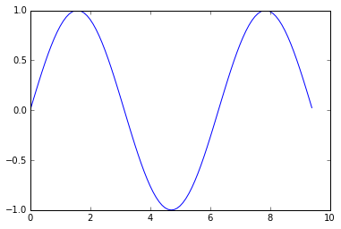
A função mais importante no matplotlib é o plot , que permite plotar dados 2D. Aqui está um exemplo simples:

 import numpy as np import matplotlib.pyplot as plt # Compute the x and y coordinates for points on a sine curve x = np . arange ( 0 , 3 * np . pi , 0.1 ) y = np . sin ( x ) # Plot the points using matplotlib plt . plot ( x , y ) plt . show () # You must call plt.show() to make graphics appear. 

Executar este código produz o seguinte gráfico:

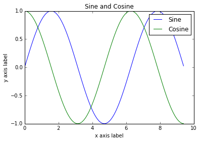
Com apenas um pouco de trabalho extra, podemos facilmente plotar várias linhas de uma vez e adicionar um título, legenda e rótulos de eixo:

 import numpy as np import matplotlib.pyplot as plt # Compute the x and y coordinates for points on sine and cosine curves x = np . arange ( 0 , 3 * np . pi , 0.1 ) y_sin = np . sin ( x ) y_cos = np . cos ( x ) # Plot the points using matplotlib plt . plot ( x , y_sin ) plt . plot ( x , y_cos ) plt . xlabel ( 'x axis label' ) plt . ylabel ( 'y axis label' ) plt . title ( 'Sine and Cosine' ) plt . legend ([ 'Sine' , 'Cosine' ]) plt . show () 

Você pode ler muito mais sobre a função de plot na documentação .

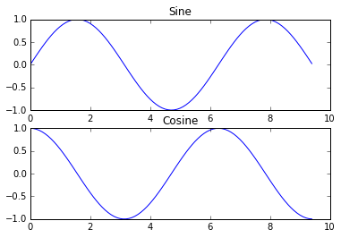
Subtramas

Você pode plotar coisas diferentes na mesma figura usando a função subplot . Aqui está um exemplo:

 import numpy as np import matplotlib.pyplot as plt # Compute the x and y coordinates for points on sine and cosine curves x = np . arange ( 0 , 3 * np . pi , 0.1 ) y_sin = np . sin ( x ) y_cos = np . cos ( x ) # Set up a subplot grid that has height 2 and width 1, # and set the first such subplot as active. plt . subplot ( 2 , 1 , 1 ) # Make the first plot plt . plot ( x , y_sin ) plt . title ( 'Sine' ) # Set the second subplot as active, and make the second plot. plt . subplot ( 2 , 1 , 2 ) plt . plot ( x , y_cos ) plt . title ( 'Cosine' ) # Show the figure. plt . show () 

Você pode ler muito mais sobre a função subplot na documentação .

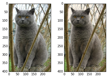
Imagens

Você pode usar a função imshow para mostrar imagens. Aqui está um exemplo:

 import numpy as np from scipy.misc import imread , imresize import matplotlib.pyplot as plt img = imread ( 'assets/cat.jpg' ) img_tinted = img * [ 1 , 0.95 , 0.9 ] # Show the original image plt . subplot ( 1 , 2 , 1 ) plt . imshow ( img ) # Show the tinted image plt . subplot ( 1 , 2 , 2 ) # A slight gotcha with imshow is that it might give strange results # if presented with data that is not uint8. To work around this, we # explicitly cast the image to uint8 before displaying it. plt . imshow ( np . uint8 ( img_tinted )) plt . show ()